Supervised Learning¶

In [1]:

suppressPackageStartupMessages(library(tidyverse))

In [2]:

options(repr.plot.width=4, repr.plot.height=4)

Regression¶

In [3]:

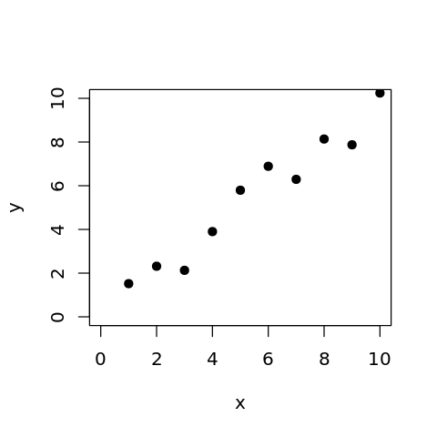
set.seed(10)

x <- 1:10
y = x + rnorm(10, 0.5, 1)

In [4]:

plot(x, y, xlim = c(0, 10), ylim = c(0, 10), pch = 19)

../_images/cliburn_Supervised_Learning_Solutions_5_0.png

Detour: Image formatting in base graphics¶

Point characters

Linear Regression¶

In [5]:

model.lm <- lm(y ~ x)

Predicting from a fitted model¶

In [6]:

predict(model.lm)

1: 1.26208403232277
2: 2.20591939228898
3: 3.14975475225518
4: 4.09359011222138
5: 5.03742547218758
6: 5.98126083215378
7: 6.92509619211998
8: 7.86893155208618
9: 8.81276691205238
10: 9.75660227201858

Predicting for new data¶

In [7]:

predict(model.lm, data.frame(x = c(1.5, 3.5, 5.5)))

1: 1.73400171230588
2: 3.62167243223828
3: 5.50934315217068

In [8]:

plot(x, y, xlim = c(0, 10), ylim = c(0, 10), pch = 19)
lines(x, predict(model.lm), col = 3)

../_images/cliburn_Supervised_Learning_Solutions_13_0.png

Alternative¶

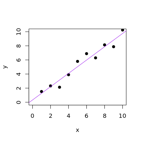
Note that abline plots the fitted line throughout the plot limits for the x-axis.

In [9]:

plot(x, y, xlim = c(0, 10), ylim = c(0, 10), pch = 19)
abline(model.lm, col="purple")

../_images/cliburn_Supervised_Learning_Solutions_15_0.png

Detour: Colors in base graphics¶

Colors

You can also used named colors - run colors to get all named colors available.

In [10]:

colors()

'white'
'aliceblue'
'antiquewhite'
'antiquewhite1'
'antiquewhite2'
'antiquewhite3'
'antiquewhite4'
'aquamarine'
'aquamarine1'
'aquamarine2'
'aquamarine3'
'aquamarine4'
'azure'
'azure1'
'azure2'
'azure3'
'azure4'
'beige'
'bisque'
'bisque1'
'bisque2'
'bisque3'
'bisque4'
'black'
'blanchedalmond'
'blue'
'blue1'
'blue2'
'blue3'
'blue4'
'blueviolet'
'brown'
'brown1'
'brown2'
'brown3'
'brown4'
'burlywood'
'burlywood1'
'burlywood2'
'burlywood3'
'burlywood4'
'cadetblue'
'cadetblue1'
'cadetblue2'
'cadetblue3'
'cadetblue4'
'chartreuse'
'chartreuse1'
'chartreuse2'
'chartreuse3'
'chartreuse4'
'chocolate'
'chocolate1'
'chocolate2'
'chocolate3'
'chocolate4'
'coral'
'coral1'
'coral2'
'coral3'
'coral4'
'cornflowerblue'
'cornsilk'
'cornsilk1'
'cornsilk2'
'cornsilk3'
'cornsilk4'
'cyan'
'cyan1'
'cyan2'
'cyan3'
'cyan4'
'darkblue'
'darkcyan'
'darkgoldenrod'
'darkgoldenrod1'
'darkgoldenrod2'
'darkgoldenrod3'
'darkgoldenrod4'
'darkgray'
'darkgreen'
'darkgrey'
'darkkhaki'
'darkmagenta'
'darkolivegreen'
'darkolivegreen1'
'darkolivegreen2'
'darkolivegreen3'
'darkolivegreen4'
'darkorange'
'darkorange1'
'darkorange2'
'darkorange3'
'darkorange4'
'darkorchid'
'darkorchid1'
'darkorchid2'
'darkorchid3'
'darkorchid4'
'darkred'
'darksalmon'
'darkseagreen'
'darkseagreen1'
'darkseagreen2'
'darkseagreen3'
'darkseagreen4'
'darkslateblue'
'darkslategray'
'darkslategray1'
'darkslategray2'
'darkslategray3'
'darkslategray4'
'darkslategrey'
'darkturquoise'
'darkviolet'
'deeppink'
'deeppink1'
'deeppink2'
'deeppink3'
'deeppink4'
'deepskyblue'
'deepskyblue1'
'deepskyblue2'
'deepskyblue3'
'deepskyblue4'
'dimgray'
'dimgrey'
'dodgerblue'
'dodgerblue1'
'dodgerblue2'
'dodgerblue3'
'dodgerblue4'
'firebrick'
'firebrick1'
'firebrick2'
'firebrick3'
'firebrick4'
'floralwhite'
'forestgreen'
'gainsboro'
'ghostwhite'
'gold'
'gold1'
'gold2'
'gold3'
'gold4'
'goldenrod'
'goldenrod1'
'goldenrod2'
'goldenrod3'
'goldenrod4'
'gray'
'gray0'
'gray1'
'gray2'
'gray3'
'gray4'
'gray5'
'gray6'
'gray7'
'gray8'
'gray9'
'gray10'
'gray11'
'gray12'
'gray13'
'gray14'
'gray15'
'gray16'
'gray17'
'gray18'
'gray19'
'gray20'
'gray21'
'gray22'
'gray23'
'gray24'
'gray25'
'gray26'
'gray27'
'gray28'
'gray29'
'gray30'
'gray31'
'gray32'
'gray33'
'gray34'
'gray35'
'gray36'
'gray37'
'gray38'
'gray39'
'gray40'
'gray41'
'gray42'
'gray43'
'gray44'
'gray45'
'gray46'
'gray47'
'gray48'
'gray49'
'gray50'
'gray51'
'gray52'
'gray53'
'gray54'
'gray55'
'gray56'
'gray57'
'gray58'
'gray59'
'gray60'
'gray61'
'gray62'
'gray63'
'gray64'
'gray65'
'gray66'
'gray67'
'gray68'
'gray69'
'gray70'
'gray71'
'gray72'
'gray73'
'gray74'
'gray75'
'gray76'
'gray77'
'gray78'
'gray79'
'gray80'
'gray81'
'gray82'
'gray83'
'gray84'
'gray85'
'gray86'
'gray87'
'gray88'
'gray89'
'gray90'
'gray91'
'gray92'
'gray93'
'gray94'
'gray95'
'gray96'
'gray97'
'gray98'
'gray99'
'gray100'
'green'
'green1'
'green2'
'green3'
'green4'
'greenyellow'
'grey'
'grey0'
'grey1'
'grey2'
'grey3'
'grey4'
'grey5'
'grey6'
'grey7'
'grey8'
'grey9'
'grey10'
'grey11'
'grey12'
'grey13'
'grey14'
'grey15'
'grey16'
'grey17'
'grey18'
'grey19'
'grey20'
'grey21'
'grey22'
'grey23'
'grey24'
'grey25'
'grey26'
'grey27'
'grey28'
'grey29'
'grey30'
'grey31'
'grey32'
'grey33'
'grey34'
'grey35'
'grey36'
'grey37'
'grey38'
'grey39'
'grey40'
'grey41'
'grey42'
'grey43'
'grey44'
'grey45'
'grey46'
'grey47'
'grey48'
'grey49'
'grey50'
'grey51'
'grey52'
'grey53'
'grey54'
'grey55'
'grey56'
'grey57'
'grey58'
'grey59'
'grey60'
'grey61'
'grey62'
'grey63'
'grey64'
'grey65'
'grey66'
'grey67'
'grey68'
'grey69'
'grey70'
'grey71'
'grey72'
'grey73'
'grey74'
'grey75'
'grey76'
'grey77'
'grey78'
'grey79'
'grey80'
'grey81'
'grey82'
'grey83'
'grey84'
'grey85'
'grey86'
'grey87'
'grey88'
'grey89'
'grey90'
'grey91'
'grey92'
'grey93'
'grey94'
'grey95'
'grey96'
'grey97'
'grey98'
'grey99'
'grey100'
'honeydew'
'honeydew1'
'honeydew2'
'honeydew3'
'honeydew4'
'hotpink'
'hotpink1'
'hotpink2'
'hotpink3'
'hotpink4'
'indianred'
'indianred1'
'indianred2'
'indianred3'
'indianred4'
'ivory'
'ivory1'
'ivory2'
'ivory3'
'ivory4'
'khaki'
'khaki1'
'khaki2'
'khaki3'
'khaki4'
'lavender'
'lavenderblush'
'lavenderblush1'
'lavenderblush2'
'lavenderblush3'
'lavenderblush4'
'lawngreen'
'lemonchiffon'
'lemonchiffon1'
'lemonchiffon2'
'lemonchiffon3'
'lemonchiffon4'
'lightblue'
'lightblue1'
'lightblue2'
'lightblue3'
'lightblue4'
'lightcoral'
'lightcyan'
'lightcyan1'
'lightcyan2'
'lightcyan3'
'lightcyan4'
'lightgoldenrod'
'lightgoldenrod1'
'lightgoldenrod2'
'lightgoldenrod3'
'lightgoldenrod4'
'lightgoldenrodyellow'
'lightgray'
'lightgreen'
'lightgrey'
'lightpink'
'lightpink1'
'lightpink2'
'lightpink3'
'lightpink4'
'lightsalmon'
'lightsalmon1'
'lightsalmon2'
'lightsalmon3'
'lightsalmon4'
'lightseagreen'
'lightskyblue'
'lightskyblue1'
'lightskyblue2'
'lightskyblue3'
'lightskyblue4'
'lightslateblue'
'lightslategray'
'lightslategrey'
'lightsteelblue'
'lightsteelblue1'
'lightsteelblue2'
'lightsteelblue3'
'lightsteelblue4'
'lightyellow'
'lightyellow1'
'lightyellow2'
'lightyellow3'
'lightyellow4'
'limegreen'
'linen'
'magenta'
'magenta1'
'magenta2'
'magenta3'
'magenta4'
'maroon'
'maroon1'
'maroon2'
'maroon3'
'maroon4'
'mediumaquamarine'
'mediumblue'
'mediumorchid'
'mediumorchid1'
'mediumorchid2'
'mediumorchid3'
'mediumorchid4'
'mediumpurple'
'mediumpurple1'
'mediumpurple2'
'mediumpurple3'
'mediumpurple4'
'mediumseagreen'
'mediumslateblue'
'mediumspringgreen'
'mediumturquoise'
'mediumvioletred'
'midnightblue'
'mintcream'
'mistyrose'
'mistyrose1'
'mistyrose2'
'mistyrose3'
'mistyrose4'
'moccasin'
'navajowhite'
'navajowhite1'
'navajowhite2'
'navajowhite3'
'navajowhite4'
'navy'
'navyblue'
'oldlace'
'olivedrab'
'olivedrab1'
'olivedrab2'
'olivedrab3'
'olivedrab4'
'orange'
'orange1'
'orange2'
'orange3'
'orange4'
'orangered'
'orangered1'
'orangered2'
'orangered3'
'orangered4'
'orchid'
'orchid1'
'orchid2'
'orchid3'
'orchid4'
'palegoldenrod'
'palegreen'
'palegreen1'
'palegreen2'
'palegreen3'
'palegreen4'
'paleturquoise'
'paleturquoise1'
'paleturquoise2'
'paleturquoise3'
'paleturquoise4'
'palevioletred'
'palevioletred1'
'palevioletred2'
'palevioletred3'
'palevioletred4'
'papayawhip'
'peachpuff'
'peachpuff1'
'peachpuff2'
'peachpuff3'
'peachpuff4'
'peru'
'pink'
'pink1'
'pink2'
'pink3'
'pink4'
'plum'
'plum1'
'plum2'
'plum3'
'plum4'
'powderblue'
'purple'
'purple1'
'purple2'
'purple3'
'purple4'
'red'
'red1'
'red2'
'red3'
'red4'
'rosybrown'
'rosybrown1'
'rosybrown2'
'rosybrown3'
'rosybrown4'
'royalblue'
'royalblue1'
'royalblue2'
'royalblue3'
'royalblue4'
'saddlebrown'
'salmon'
'salmon1'
'salmon2'
'salmon3'
'salmon4'
'sandybrown'
'seagreen'
'seagreen1'
'seagreen2'
'seagreen3'
'seagreen4'
'seashell'
'seashell1'
'seashell2'
'seashell3'
'seashell4'
'sienna'
'sienna1'
'sienna2'
'sienna3'
'sienna4'
'skyblue'
'skyblue1'
'skyblue2'
'skyblue3'
'skyblue4'
'slateblue'
'slateblue1'
'slateblue2'
'slateblue3'
'slateblue4'
'slategray'
'slategray1'
'slategray2'
'slategray3'
'slategray4'
'slategrey'
'snow'
'snow1'
'snow2'
'snow3'
'snow4'
'springgreen'
'springgreen1'
'springgreen2'
'springgreen3'
'springgreen4'
'steelblue'
'steelblue1'
'steelblue2'
'steelblue3'
'steelblue4'
'tan'
'tan1'
'tan2'
'tan3'
'tan4'
'thistle'
'thistle1'
'thistle2'
'thistle3'
'thistle4'
'tomato'
'tomato1'
'tomato2'
'tomato3'
'tomato4'
'turquoise'
'turquoise1'
'turquoise2'
'turquoise3'
'turquoise4'
'violet'
'violetred'
'violetred1'
'violetred2'
'violetred3'
'violetred4'
'wheat'
'wheat1'
'wheat2'
'wheat3'
'wheat4'
'whitesmoke'
'yellow'
'yellow1'
'yellow2'
'yellow3'
'yellow4'
'yellowgreen'

Polynomial Regression¶

In [11]:

model.poly5 <- lm(y ~ poly(x, 5))

In [12]:

plot(x, y, xlim = c(0, 10), ylim = c(0, 10), pch = 19)
lines(x, predict(model.poly5), col = "orange")

../_images/cliburn_Supervised_Learning_Solutions_20_0.png

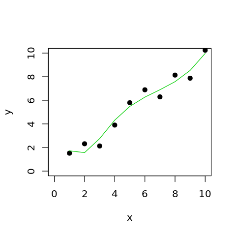
Spline Regression¶

Splines are essentially piecewise polynomial fits. There are two parameters

degree determines the type of piecewise polynomials used (e.g. degree=3 uses cubic polynomials)
knots are where the piecewise polynomials meet (determine number of pieces)

In [13]:

library(splines)

In [14]:

model.spl <- lm(y ~ bs(x, degree=3, knots=4))

In [15]:

plot(x, y, xlim = c(0, 10), ylim = c(0, 10), pch = 19)
lines(x, predict(model.spl), col = 3)

../_images/cliburn_Supervised_Learning_Solutions_24_0.png

Connect the dots¶

In [16]:

plot(x, y, xlim = c(0, 10), ylim = c(0, 10), pch = 19)
lines(x, y, col="red")

../_images/cliburn_Supervised_Learning_Solutions_26_0.png

Classification¶

In [17]:

levels(iris$Species)

'setosa'
'versicolor'
'virginica'

In [18]:

df <- iris %>% filter(Species != "setosa")
df$Species <- droplevels(df$Species)

In [19]:

options(repr.plot.width=8, repr.plot.height=4)
par(mfrow=c(1,2))
plot(df[,1], df[,2], col=as.integer(df$Species))
plot(df[,3], df[,4], col=as.integer(df$Species))

../_images/cliburn_Supervised_Learning_Solutions_31_0.png

In [20]:

sample.int(10, 5)

9
6
7
3
8

Split into 50% training and 50% test sets¶

In [21]:

library(class)

In [22]:

set.seed(10)
sample <- sample.int(n = nrow(df), size = floor(.5*nrow(df)), replace = F)
train <- df[sample, 1:4]
test  <- df[-sample, 1:4]
train.cls = df$Species[sample]
test.cls = df$Species[-sample]

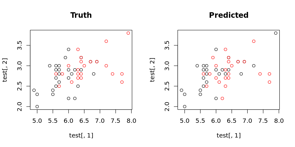
In [23]:

test.pred <- knn(train, test, train.cls, k = 3)

In [24]:

options(repr.plot.width=8, repr.plot.height=4)
par(mfrow=c(1,2))
plot(test[,1], test[,2], col=as.integer(test.cls), main="Truth")
plot(test[,1], test[,2], col=as.integer(test.pred), main="Predicted")

../_images/cliburn_Supervised_Learning_Solutions_37_0.png

In [25]:

table(test.pred, test.cls)

test.cls
test.pred    versicolor virginica
  versicolor         25         0
  virginica           3        22

Logistic Regression¶

In [26]:

head(train)

	Sepal.Length	Sepal.Width	Petal.Length	Petal.Width
51	6.3	3.3	6.0	2.5
31	5.5	2.4	3.8	1.1
42	6.1	3.0	4.6	1.4
68	7.7	3.8	6.7	2.2
9	6.6	2.9	4.6	1.3
22	6.1	2.8	4.0	1.3

The warning is due to the fact that vanilla logistic regression does not like perfectly separated data sets. The usual remedy is to add a penalization factor.

In [27]:

model.logistic <- glm(train.cls ~ .,
                      family=binomial(link='logit'), data=train)

Warning message:
“glm.fit: algorithm did not converge”Warning message:
“glm.fit: fitted probabilities numerically 0 or 1 occurred”

In [28]:

summary(model.logistic)

Call:
glm(formula = train.cls ~ ., family = binomial(link = "logit"),
    data = train)

Deviance Residuals:
       Min          1Q      Median          3Q         Max
-2.347e-05  -2.110e-08   2.110e-08   2.110e-08   2.792e-05

Coefficients:
               Estimate Std. Error z value Pr(>|z|)
(Intercept)   1.658e+00  1.263e+06   0.000    1.000
Sepal.Length -6.152e+01  9.061e+04  -0.001    0.999
Sepal.Width  -8.214e+01  4.829e+05   0.000    1.000
Petal.Length  7.759e+01  1.673e+05   0.000    1.000
Petal.Width   1.453e+02  2.148e+05   0.001    0.999

(Dispersion parameter for binomial family taken to be 1)

    Null deviance: 6.8593e+01  on 49  degrees of freedom
Residual deviance: 2.0984e-09  on 45  degrees of freedom
AIC: 10

Number of Fisher Scoring iterations: 25

In [29]:

test.pred <- ifelse(predict(model.logistic, test) < 0, 1, 2)

In [30]:

options(repr.plot.width=8, repr.plot.height=4)
par(mfrow=c(1,2))
plot(test[,1], test[,2], col=as.integer(test.cls), main="Truth")
plot(test[,1], test[,2], col=test.pred, main="Predicted")

../_images/cliburn_Supervised_Learning_Solutions_45_0.png

In [31]:

table(test.pred, test.cls)

test.cls
test.pred versicolor virginica
        1         24         3
        2          4        19

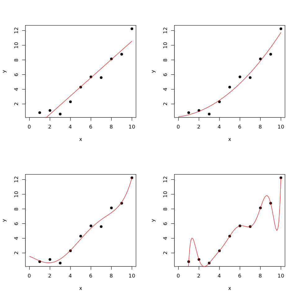
Overfitting¶

In [32]:

set.seed(10)

x <- 1:10
y = 0.1*x^2 + 0.2*x + rnorm(10, 0.5, 1)

In [33]:

m1 <- lm(y ~ x)
m2 <- lm(y ~ poly(x, 2))
m5 <- lm(y ~ poly(x, 5))
m9 <- lm(y ~ poly(x, 9))

In [34]:

options(repr.plot.width=8, repr.plot.height=8)

xp = seq(0, 10, length.out = 100)
df <- data.frame(x=xp)

par(mfrow=c(2,2))
plot(x, y, xlim = c(0, 10), pch = 19)
lines(xp, predict(m1, df), col = "red")
plot(x, y, xlim = c(0, 10), pch = 19)
lines(xp, predict(m2, df), col = "red")
plot(x, y, xlim = c(0, 10), pch = 19)
lines(xp, predict(m5, df), col = "red")
plot(x, y, xlim = c(0, 10), pch = 19)
lines(xp, predict(m9, df), col = "red")

../_images/cliburn_Supervised_Learning_Solutions_50_0.png

In [35]:

for (model in list(m1, m2, m5, m9)) {
    print(round(sum((predict(model, data.frame(x=x)) - y)^2), 2))
    }

[1] 9.18
[1] 4.15
[1] 2.09
[1] 0

In [36]:

test.x <- runif(10, 0, 10)
test.y <- 0.1*test.x^2 + 0.2*test.x + rnorm(10, 0.5, 3)

In [37]:

for (model in list(m1, m2, m5, m9)) {
    print(round(sum((predict(model, data.frame(x=test.x)) - test.y)^2), 2))
    }

[1] 112.25
[1] 103.79
[1] 99.8
[1] 111.98

Cross-validation¶

In [38]:

for (k in 1:5) {
    rss <- 0
    for (i in 1:10) {
        xmo <- x[-i]
        ymo <- y[-i]
        model <- lm(ymo ~ poly(xmo, k))
        res <- (predict(model, data.frame(xmo=x[i])) - y[i])^2
        rss <- rss + res
    }
    print(k)
    print(rss)
}

Feature Selection¶

In [39]:

suppressPackageStartupMessages(library(genefilter))

In [40]:

set.seed(123)
n = 20
m = 1000
EXPRS = matrix(rnorm(2 * n * m), 2 * n, m)
rownames(EXPRS) = paste("pt", 1:(2 * n), sep = "")
colnames(EXPRS) = paste("g", 1:m, sep = "")
grp = as.factor(rep(1:2, c(n, n)))

In [41]:

head(EXPRS, 3)

	g1	g2	g3	g4	g5	g6	g7	g8	g9	g10	⋯	g991	g992	g993	g994	g995	g996	g997	g998	g999	g1000
pt1	-0.5604756	-0.6947070	0.005764186	0.1176466	1.052711	2.1988103	-0.7886220	-1.6674751	0.2374303	-0.2052993	⋯	0.3780725	1.974814	-0.4535280	-0.4552866	-2.3004639	-0.3804398	0.2870161	-0.2018602	-1.6727583	1.1379048
pt2	-0.2301775	-0.2079173	0.385280401	-0.9474746	-1.049177	1.3124130	-0.5021987	0.7364960	1.2181086	0.6511933	⋯	0.5981352	-1.021826	-2.0371182	1.5636880	-0.9501855	0.6671640	-0.6702249	1.1181721	-0.5414325	1.2684239
pt3	1.5587083	-1.2653964	-0.370660032	-0.4905574	-1.260155	-0.2651451	1.4960607	0.3860266	-1.3387743	0.2737665	⋯	0.5774870	0.853561	-0.3030158	-0.1434414	-0.8478627	0.2413405	-0.5417177	0.1625707	0.1995339	0.0427062

In [42]:

stats = abs(rowttests(t(EXPRS), grp)$statistic)

In [43]:

head(stats,3)

0.674624258566226
0.741717473727548
3.02542265710511

In [44]:

ii <- order(-stats)

In [45]:

TOPEXPRS <- EXPRS[, ii[1:10]]

In [46]:

mod0 = knn(train = TOPEXPRS, test = TOPEXPRS, cl = grp, k = 3)
table(mod0, grp)

Note: Feature selection is not part of the CV process, and so the results are OVER-OPTIMISTIC

In [47]:

mode1 = knn.cv(TOPEXPRS, grp, k = 3)
table(mode1, grp)

grp
mode1  1  2
    1 16  0
    2  4 20

In [48]:

suppressPackageStartupMessages(library(multtest))

In [49]:

top.features <- function(EXP, resp, test, fsnum) {
     top.features.i <- function(i, EXP, resp, test, fsnum) {
         stats <- abs(mt.teststat(EXP[, -i], resp[-i], test = test))
         ii <- order(-stats)[1:fsnum]
         rownames(EXP)[ii]
    }
    sapply(1:ncol(EXP), top.features.i,
           EXP = EXP, resp = resp, test = test, fsnum = fsnum)
}

In [50]:

# This function evaluates the knn
knn.loocv <- function(EXP, resp, test, k, fsnum, tabulate = FALSE, permute = FALSE) {
    if (permute) {
        resp = sample(resp)
        }
    topfeat = top.features(EXP, resp, test, fsnum)
    pids = rownames(EXP)
    EXP = t(EXP)
    colnames(EXP) = as.character(pids)
    knn.loocv.i = function(i, EXP, resp, k, topfeat) {
    ii = topfeat[, i]
    mod = knn(train = EXP[-i, ii], test = EXP[i, ii], cl = resp[-i], k = k)[1] }
    out = sapply(1:nrow(EXP), knn.loocv.i,
                 EXP = EXP, resp = resp, k
                 = k, topfeat = topfeat)
    if (tabulate)
        out = ftable(pred = out, obs = resp)
    return(out)
}

Reminder of what the data look like¶

In [51]:

EXPRS[1:5, 1:5]

	g1	g2	g3	g4	g5
pt1	-0.56047565	-0.6947070	0.005764186	0.1176466	1.0527115
pt2	-0.23017749	-0.2079173	0.385280401	-0.9474746	-1.0491770
pt3	1.55870831	-1.2653964	-0.370660032	-0.4905574	-1.2601552
pt4	0.07050839	2.1689560	0.644376549	-0.2560922	3.2410399
pt5	0.12928774	1.2079620	-0.220486562	1.8438620	-0.4168576

In [52]:

levels(grp)

'1'
'2'

In [53]:

knn.loocv(t(EXPRS), grp, "t.equalvar", 3, 10, TRUE)

obs  1  2
pred
1         7  7
2        13 13

Cross-validation done right (simple version)¶

In [54]:

pred <- numeric(2*n)
for (i in 1:(2*n)) {
    stats = abs(rowttests(t(EXPRS[-i,]), grp[-i])$statistic)
    ii <- order(-stats)
    TOPEXPRS <- EXPRS[-i, ii[1:10]]
    pred[i] = knn(TOPEXPRS, EXPRS[i, ii[1:10]], grp[-i], k = 3)
}

In [55]:

table(pred, grp)

Exercise¶

Repeat the last experiment with a noisy quantitative outcome
First simulate a data matrix of dimension n = 50 (patients) and m (genes)
Next draw the outcome for n=50 patients from a standard normal distribution independent of the data matrix
There is no relationship between the expressions and the outcome (by design)
We consider m=45 and m=50000
We conduct Naive LOOCV using the top 10 features

Data Generation¶

In [56]:

set.seed(123)
n <- 50
m <- 50000
EXPRS <- matrix(rnorm(n*m), n, m)
rownames(EXPRS) = paste("pt", 1:n, sep = "")
colnames(EXPRS) = paste("g", 1:m, sep = "")
OUTCOMES <- rnorm(n)

Proper cross-validation¶

In [57]:

pred0 <- numeric(n)
for (i in 1:n) {

    stats <- abs(cor(OUTCOMES[-i], EXPRS[-i,]))
    ii <- order(-stats)
    TOPEXPRS <- EXPRS[, ii[1:10]]

    data <- data.frame(y = OUTCOMES, x = I(TOPEXPRS))
    model <- lm(y ~ x, data=data[-i,])
    pred0[i] <- predict(model, data[i,])
}

Naive cross-validation¶

In [58]:

stats <- abs(cor(OUTCOMES, EXPRS))
ii <- order(-stats)
TOPEXPRS <- EXPRS[, ii[1:10]]

In [59]:

pred <- numeric(n)
for (i in 1:n) {
    data <- data.frame(y = OUTCOMES, x = I(TOPEXPRS))
    model <- lm(y ~ x, data=data[-i,])
    pred[i] <- predict(model, data[i,])
}

In [60]:

plot(OUTCOMES, pred, col='red', xlab="Observed Values", ylab="Predicted Values")
points(OUTCOMES, pred.0, pch=4, col='blue')
abline(lm(pred ~ OUTCOMES), col='red')

Error in xy.coords(x, y): object 'pred.0' not found
Traceback:

1. points(OUTCOMES, pred.0, pch = 4, col = "blue")
2. points.default(OUTCOMES, pred.0, pch = 4, col = "blue")
3. plot.xy(xy.coords(x, y), type = type, ...)
4. xy.coords(x, y)

../_images/cliburn_Supervised_Learning_Solutions_89_1.png